Aplot Tutorial

Creating a graph from Fortran using Aplot is simple and easy. This tutorial is meant to provide the necessary steps for getting started with Aplot.

Including the Module

Aplot is accessible via a single Fortran 90 module:

use aplot

Simply Fortran will take care of everything else necessary to include the Aplot library in an executable.

Initializing a Plot

The first step in creating a plot is to initialize a plot variable:

type(aplot_t)::p
...
    p = initialize_plot()

The call above creates a plot variable that is used in all subsequent calls to Aplot’s programming interface. At this point, the user may want to set up a plot title:

   call set_title(p, 'Example Plot')

At this point, no data has been added.

Adding a Data Set

Aplot can produce a handful of two-dimensional plots to visualize user data. In this example, some static data is used:

real, dimension(10)::x = (/ 1.0, 2.0, 3.0, 4.0, 5.0, 6.0, 7.0, 8.0, 9.0, 10.0 /)
real, dimension(10)::y = (/ 2.0, 4.0, 6.0, 8.0, 6.0, 4.0, 2.0, 0.0, 2.0, 4.0 /)
...
    call add_dataset(p, x, y)

The data above should now be added to the plot as a series. As mentioned in the reference section, the numbering for referencing series is zero-based. To add a label and configure our data to appear in a scatter chart, we would call:

     call set_serieslabel(p, 0, "Example Data");
    call set_seriestype(p, 0, APLOT_STYLE_DOT); 

Note that the series is refered to as 0 since it is the first data set. Another data set can be added and configured similarly, and it would be referenced using 1 as it’s index.

Depending on the data, the user might prefer to use a line plot, bar chart, or the pixel plot. The pixel plot, like the scatter plot above, uses points for each datapoint, but the smaller pixel representation might be preferable when a substantial amount of data is being drawn.

Labeling the Axes

A proper plot should always have labeled axes. In our case, we can use the following:

   call set_xlabel(p, "Easy");
    call set_ylabel(p, "Hard");

Our axes should now appear properly labeled. We could additionally set scaling on the axes, but the default behavior to autoscale the axes should be sufficient in many cases.

Display the Plot

Now that the plot is completely configured, we can actually display the plot:

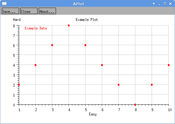
   call display_plot(p)

The call above will open a window and pause the user’s program execution until closed. In our example, it should appear as:

The appearance of the window will obviously differ depending on the platform (the example is from GNU/Linux).

Cleanup

After the window is closed, the user’s program will continue execution. In most cases, the calling routine should clean up the plot variable before moving on with the simple call:

   call destroy_plot(p)

Complete Program

The complete code to show the example plot is quite terse. To experiment, users can start with the code below:

program test
use aplot
implicit none

type(aplot_t)::p
real, dimension(10)::x = (/ 1.0, 2.0, 3.0, 4.0, 5.0, 6.0, 7.0, 8.0, 9.0, 10.0 /)
real, dimension(10)::y = (/ 2.0, 4.0, 6.0, 8.0, 6.0, 4.0, 2.0, 0.0, 2.0, 4.0 /)

    p = initialize_plot()
    call add_dataset(p, x, y)
    call set_xlabel(p, "Easy")
    call set_ylabel(p, "Hard")
    call set_title(p, "Example Plot")
    call set_serieslabel(p, 0, "Example Data")
    call set_seriestype(p, 0, APLOT_STYLE_DOT)
    call display_plot(p)
    call destroy_plot(p)

end program test