A Quick LAPACK Example

With the release of Simply Fortran 2.37, LAPACK and BLAS routines are now easily available on all supported platforms. LAPACK, or Linear Algebra Package, provides an enormous collection of subroutines for dealing with many types of matrix operations and linear systems , while BLAS, or Basic Linear Algebra Subprograms, provides lower level vector and matrix math operations. Both libraries are extremely common within scientific computing, and their inclusion with Simply Fortran should improve productivity for many of our users.

This quick example will look at solving an overdetermined system via a least-squares regression. LAPACK provides a number of routines supporting least squares operation, and this example uses SGELS, a single-precision generalized least squares solver. First, though, we'll need some sample data...

For those familiar with the sport of soccer (or football outside of the United States of America), one might expect that a correlation exists between the number of shots taken and the number of goals scored by any given player. It would be impossible to score, in fact, if no shots are taken. With the proper statistics, we can actually estimate the the percentage of goals resulting from a single player's total number of shots.

The National Womens Soccer League, or NWSL, is a professional soccer league within the United States, and it started reliably tracking player statistics during its 2016 season. The data is readily available here. Amongst the plethora of data are two sets we would need, shots taken and goals scored by each player. With some minor spreadsheet manipulation, we can build a single text file that contains the number of shots taken by each player and the corresponding number of goals scored by said player over the course of the NWSL 2016 season. We can eliminate players who did not take any shots since they don't really conform to our analysis. The simple data file can be downloaded here: nwsl2016.txt

We first need a simple subroutine to load the data into two arrays of type REAL for LAPACK to analyze. Our routine will also assign a variable with the number of data points to allow dimensioning some additional arrays before our analysis begins. The variables n, totalshots, and goals are defined in the main program, but are within the scope of this subroutine:

! Simply loads the NWSL data from a text file
subroutine loaddata()
implicit none

    integer::row_shots, row_goals
    integer::i

    open(unit=100, file='nwsl2016.txt', status='old')

    ! Two header rows
    read(100, *)
    read(100, *)

    ! First number is the number of data points
    read(100, *) n

    ! Allocate data arrays
    allocate(totalshots(n), goals(n))

    ! Load each data point as integers and re-store
    ! them in our arrays as REAL values
    do i = 1, n
        read(100, *) row_shots, row_goals
        totalshots(i) = real(row_shots)
        goals(i) = real(row_goals)
    end do

    close(100)

end subroutine loaddata

The loading routine is not particularly interesting, so we can continue to our actual least squares analysis with the data properly loaded.

To calculate our least squares fit, we need to configure two major arrays. The overdetermined system we're attempting to solve is defined simply as:

A*x = b

Our A matrix will contain the total shots taken data. Since we also want to calculate a y-intercept in this linear regression, though, our A matrix should have two columns and n rows. The first column of A, in order to properly sove for the intercept, should be entirely set to 1.0. We also need a b matrix containing our goals scored data. This matrix will only have a single column, but we need to create a new array rather than using our original data array directly. The SGELS subroutine will modify the data in both A and b in the course of its operations, so it's often desirable to create arrays just for this task, leaving the original data untouched. Our program is now:

program shots
use aplot
implicit none

    integer::n
    real, dimension(:), allocatable::totalshots, goals

    ! Arrays for calling LAPACK's SGELS driver
    real, dimension(:,:), allocatable::bdata, adata
    real, dimension(:), allocatable::work
    integer::info

    ! First, load all our data
    call loaddata()

    ! The 'n' variable now holds the number of data points,
    ! and our totalshots and goals arrays should be properly
    ! dimensioned and populated.

    ! Build arrays for LAPACK calls
    allocate(adata(n,2), bdata(n,1), work(2*n))
    adata(:,1) = 1.0             ! So an intercept is calculated
    adata(:,2) = totalshots      ! Total shots
    bdata(:,1) = goals           ! Goals

The work array is simply necessary to call SGELS.

The call to SGELS itself can appear daunting, but we've organized our inputs for this simple problem relatively well. The SGELS call becomes:

! Perform a least squares fit - documentation at:
call SGELS('N', &   ! TRANS
           n, &     ! M
           2, &     ! N
           1, &     ! NRHS 
           adata, & ! A
           n, &     ! LDA
           bdata, & ! B
           n, &     ! LDB
           work, &  ! WORK
           2*n, &   ! LWORK
           info)

The first input, 'N', specifies that the arrays are normal as opposed to transposed. The remaining scalar inputs basically deal with the dimensions of our arrays. While we might be able to explain each, the LAPACK documentation does a far superior job.

If all goes according to plan, the value after calling SGELS should be zero. We can add some print statements to generate some output as well:

Print *, "Result (0=success): ", info
Print *, "Intercept: ", bdata(1,1)
Print *, "Slope: ", bdata(2,1)

Before we try to compile this program, we need to enable LAPACK and BLAS linking. In the Project Options window under the "Linker" tab, there is a new option to enable LAPACK and BLAS linking:

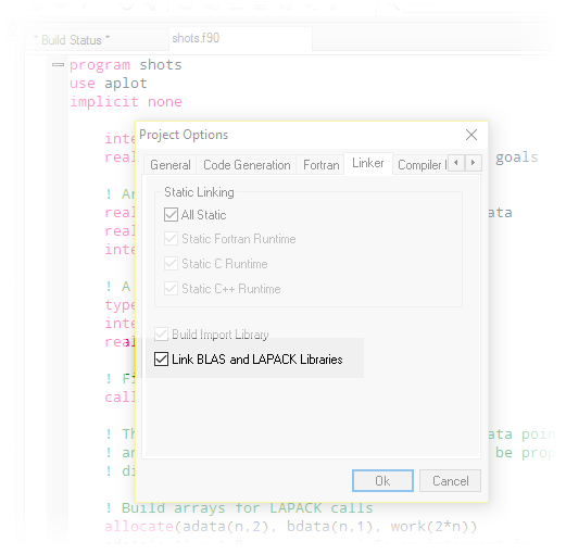
After enabling this option and saving the project, this program should run just fine, producing the following output:

Result (0=success):            0
Intercept:  -0.338190973    
Slope:   0.126037121

Based on this data, about 13% of shots taken result in a goal. The negative intercept reflects the fact that, just because a shot was taken, a goal isn't garaunteed. Multiple players have numerous shots without ever having scored.

We haven't really considered the "quality" of this linear regression by computing an R^2 value or computing t-scores for our two coefficients. Since this task is merely a demonstration, though, we might be more interested in plotting the resulting linear regression versus actual data. Luckily, Simply Fortran includes the Aplot plotting library for just such a reason. While we already have our original data, we'll need to compute regression data from our results:

type(aplot_t)::p
integer::i
real, dimension(:), allocatable::fitdata

...

! Generate regression data for each totalshots point
allocate(fitdata(n))
do i = 1, n
    fitdata(i) = bdata(1,1) + totalshots(i)*bdata(2,1)
end do

Plotting both on the same plot is straightforward:

! Plot the results
p = initialize_plot()

call add_dataset(p, totalshots, goals)
call set_seriestype(p, 0, APLOT_STYLE_DOT)
call set_serieslabel(p, 0, "Player Data")

call add_dataset(p, totalshots, fitdata)
call set_seriestype(p, 1, APLOT_STYLE_LINE)
call set_serieslabel(p, 1, "Linear Fit")

call set_xlabel(p, "Total Shots")
call set_ylabel(p, "Goals Scored")

call set_title(p, "NWSL 2016: Total Shots vs. Goals Scored")

call display_plot(p)
call destroy_plot(p)

After adding this to our program, we can now visualize our little analysis:

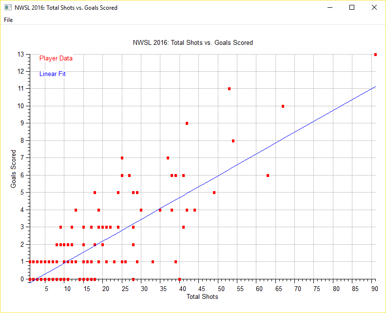
This little tutorial is meant to demonstrate the presence of LAPACK within Simply Fortran's latest version. Everything needed to replicate this is linked below:

• Data file: nwsl2016.txt
• Source Code: shots.f90

We're always open to suggestions on how Simply Fortran can better serve its users, so please feel free to contact us on the forums if you'd like to see some additions to the Simply Fortran suite.